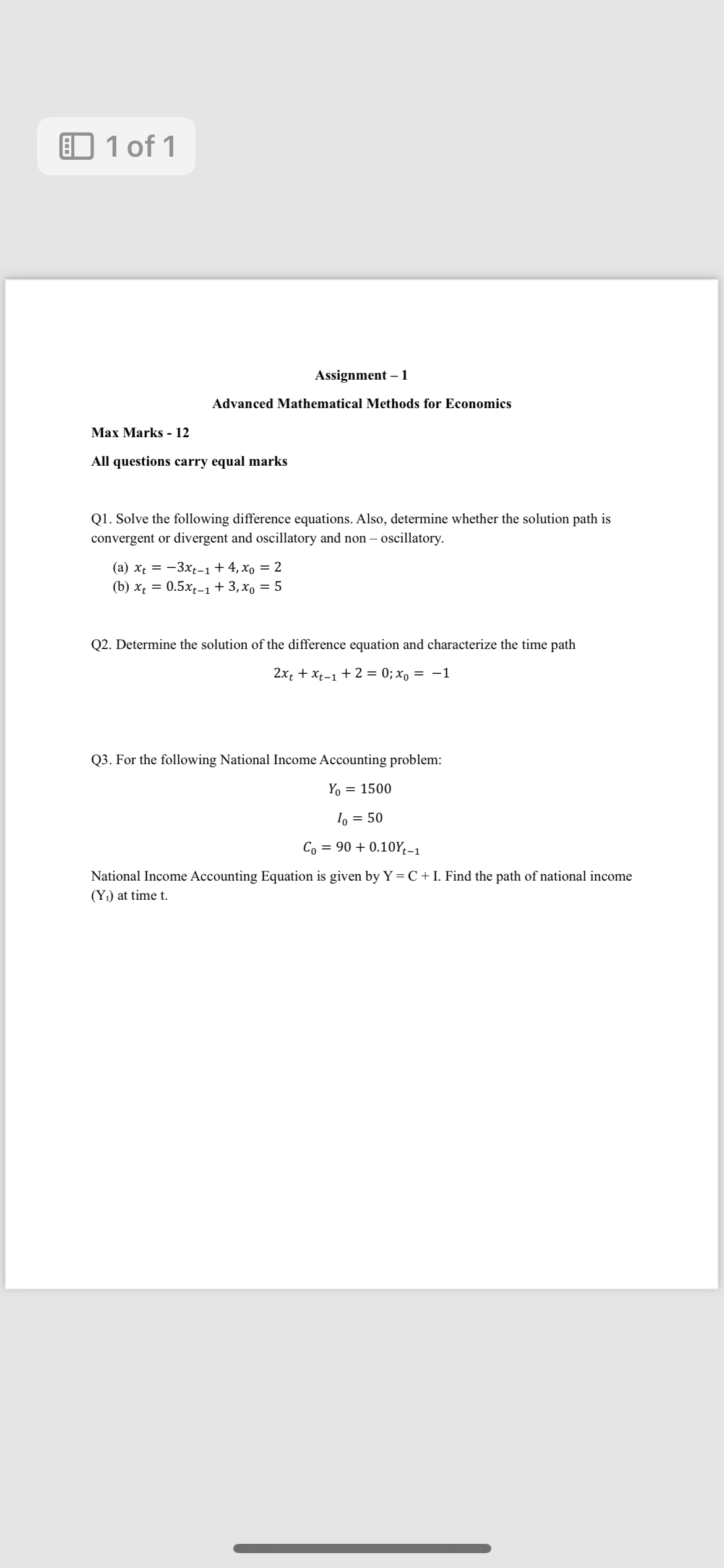
Solve the following difference equations. Also, determine whether the solution path is convergent or divergent and oscillatory and non-oscillatory. 1. xt = -3xt-1 + 4, x0 = 2; 2. x... Solve the following difference equations. Also, determine whether the solution path is convergent or divergent and oscillatory and non-oscillatory. 1. xt = -3xt-1 + 4, x0 = 2; 2. xt = 0.5xt-1 + 3, x0 = 5. Determine the solution of the difference equation 2xt + xt-1 + 2 = 0; x0 = -1. For the National Income Accounting problem with Y0 = 1500, I0 = 50, C0 = 90 + 0.10Yt-1, find the path of national income (Yt) at time t.

Understand the Problem
The question is asking for the solutions to certain difference equations, including determining their characteristics (convergent, divergent, oscillatory) and finding the path of national income over time based on an accounting equation.
Answer
- Divergent, oscillatory - Convergent, non-oscillatory (6) - Oscillatory, convergent (-1) - National income converges to approximately $155.56$.
Answer for screen readers
- For ( x_t = -3x_{t-1} + 4 ), the solution diverges and is oscillatory.
- For ( x_t = 0.5x_{t-1} + 3 ), the solution converges and is non-oscillatory; it converges to 6.
- For ( 2x_t + x_{t-1} + 2 = 0 ), the solution oscillates and converges toward -1.
- For the national income path ( Y_t ), it approaches approximately ( 155.56 ).
Steps to Solve
-
Solve the first difference equation: ( x_t = -3x_{t-1} + 4 )
To solve this equation, we will use iteration.
Start with ( x_0 = 2 ):
[ x_1 = -3 \cdot 2 + 4 = -6 + 4 = -2 ]
Next, use ( x_1 ):
[ x_2 = -3 \cdot (-2) + 4 = 6 + 4 = 10 ]
Now, use ( x_2 ):
[ x_3 = -3 \cdot 10 + 4 = -30 + 4 = -26 ]
Observing the trend, the solution diverges.
-
Determine the oscillation and convergence of the first equation
The factor of -3 indicates that the solution is oscillatory and divergent.
-
Solve the second difference equation: ( x_t = 0.5x_{t-1} + 3 )
Start with ( x_0 = 5 ):
[ x_1 = 0.5 \cdot 5 + 3 = 2.5 + 3 = 5.5 ]
Next, use ( x_1 ):
[ x_2 = 0.5 \cdot 5.5 + 3 = 2.75 + 3 = 5.75 ]
Continuing this pattern, we observe that the sequence converges to 6.
-
Determine oscillation and convergence of the second equation
Since ( 0.5 < 1 ), the solution converges and is non-oscillatory.
-
Solve for the equation ( 2x_t + x_{t-1} + 2 = 0 )
Rearranging gives:
[ x_t = -\frac{1}{2}x_{t-1} - 1 ]
Starting with ( x_0 = -1 ):
[ x_1 = -\frac{1}{2} \cdot (-1) - 1 = \frac{1}{2} - 1 = -\frac{1}{2} ]
Now for ( x_2 ):
[ x_2 = -\frac{1}{2} \cdot (-\frac{1}{2}) - 1 = \frac{1}{4} - 1 = -\frac{3}{4} ]
This shows it oscillates and converges toward -1.
-
Determine the path of national income ( Y_t )
The equation is ( Y_t = C + I = (90 + 0.1Y_{t-1}) + I_0 ).
Substitute ( I_0 = 50 ):
[ Y_t = (90 + 0.1Y_{t-1}) + 50 = 140 + 0.1Y_{t-1} ]
The steady state can be found by setting ( Y_t = Y_{t-1} = Y ):
[ Y = 140 + 0.1Y \implies 0.9Y = 140 \implies Y = \frac{140}{0.9} \approx 155.56 ]
Therefore, ( Y_t ) approaches approximately 155.56 over time.
- For ( x_t = -3x_{t-1} + 4 ), the solution diverges and is oscillatory.
- For ( x_t = 0.5x_{t-1} + 3 ), the solution converges and is non-oscillatory; it converges to 6.
- For ( 2x_t + x_{t-1} + 2 = 0 ), the solution oscillates and converges toward -1.
- For the national income path ( Y_t ), it approaches approximately ( 155.56 ).
More Information
The behavior of the difference equations can indicate stability of economic models, where divergent solutions may suggest instability while convergent solutions can indicate equilibrium. The national income accounting model illustrates how income adjusts over time based on consumption and investment.
Tips
- Not iterating enough steps to identify convergence or divergence.
- Misunderstanding the implications of factors in the recursive equations (e.g., confusing signs).
AI-generated content may contain errors. Please verify critical information