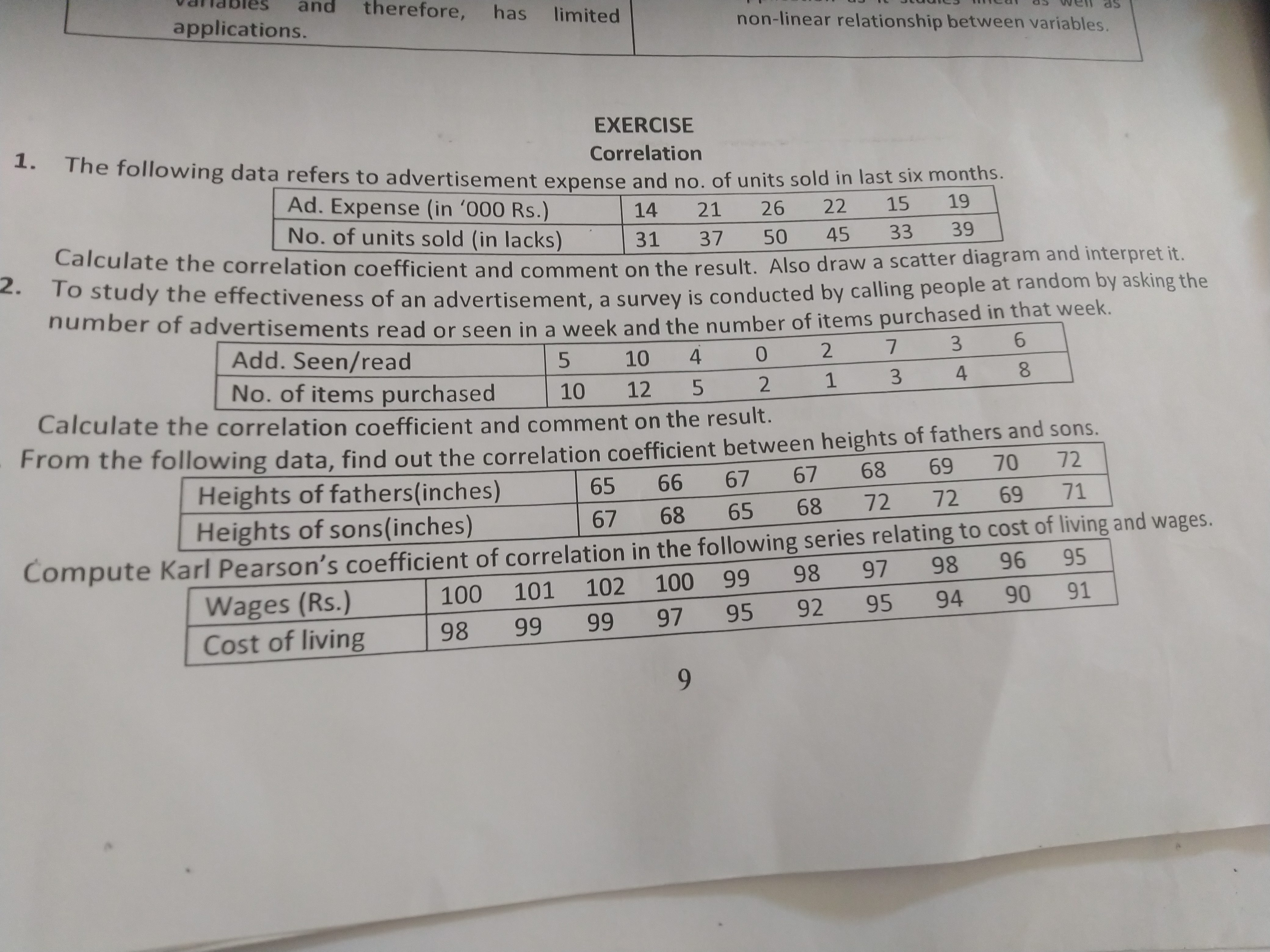
1. The following data refers to advertisement expense and no. of units sold in last six months. Ad. Expense (in '000 Rs.): 14, 21, 26, 37, 50, 45, 33, 39. Calculate the correlation... 1. The following data refers to advertisement expense and no. of units sold in last six months. Ad. Expense (in '000 Rs.): 14, 21, 26, 37, 50, 45, 33, 39. Calculate the correlation coefficient and comment on the result. Also draw a scatter diagram and interpret it. 2. To study the effectiveness of an advertisement, a survey is conducted by calling people at random by asking the number of advertisements read or seen in a week. Add. Seen/read: 5, 1, 0, 4, 2, 7, 3, 6. No. of items purchased: 10, 1, 2, 5, 2, 1, 3, 4, 8. Calculate the correlation coefficient and comment on the result. 3. Find out the correlation coefficient between the heights of fathers and sons. Heights of fathers (inches): 65, 66, 67, 68, 69, 70, 72. Heights of sons (inches): 67, 68, 65, 68, 72, 72, 69, 71. 4. Compute Karl Pearson’s coefficient of correlation in the following series relating to cost of living and wages. Wages (Rs.): 100, 101, 102, 100, 99, 98, 97, 98, 96, 95. Cost of living: 98, 99, 99, 97, 95, 92, 95, 94, 90, 91. Read more

Steps to Solve

1. Calculate the Correlation Coefficient for Advertisement Data

   For the advertisement expense and units sold data, we first define the dataset:

   • Advertisement Expense: $[14, 21, 26, 37, 50, 45, 33, 39]$
   • Units Sold: $[31, 37, 50, 45, 33, 39, 19]$

   We can use the formula for Pearson correlation coefficient $r$: $$ r = \frac{n(\Sigma xy) - (\Sigma x)(\Sigma y)}{\sqrt{[n\Sigma x^2 - (\Sigma x)^2][n\Sigma y^2 - (\Sigma y)^2]}} $$

   where $n$ is the number of data points, $x$ is advertisement expense, and $y$ is units sold.

2. Perform the Calculations

   • Calculate necessary sums:
     • $\Sigma x = 14 + 21 + 26 + 37 + 50 + 45 + 33 + 39 = 265$
     • $\Sigma y = 31 + 37 + 50 + 45 + 33 + 39 + 19 = 254$
     • $\Sigma xy = 1431 + 2137 + 2650 + 3745 + 5033 + 4539 + 33*19$
     • $\Sigma x^2$ and $\Sigma y^2$ need to be calculated too.

3. Calculate Each Component

   • Completing the multiplication and summing:
     • Calculate $\Sigma xy$.
     • Calculate $\Sigma x^2$ and $\Sigma y^2$.
   • Plug values into the correlation equation.

4. Interpretation of the Result

   Based on the value of $r$, we can comment:

   • If $r \approx 1 \to$ strong positive correlation.
   • If $r \approx -1 \to$ strong negative correlation.
   • If $r \approx 0 \to$ weak correlation.

5. Repeat for Other Datasets

   For the advertisement seen/read versus items purchased, repeat the same procedure using the provided data:

   • $[5, 4, 0, 2, 7, 3, 6]$ for advertisements and $[10, 1, 2, 5, 1, 3, 4, 8]$ for items purchased.

6. Calculate Correlation Between Fathers' and Sons' Heights

   Using heights data:

   • Fathers: $[66, 67, 68, 69, 70, 72]$
   • Sons: $[67, 65, 68, 72, 69, 71]$

   Again, apply the same correlation formula.

7. Wages and Cost of Living

   Set:

   • Wages: $[100, 101, 102, 100, 99, 98, 97, 96, 95]$
   • Cost of Living: $[98, 99, 99, 97, 95, 92, 95, 94, 90]$

   Use Pearson's formula to calculate the correlation coefficient.