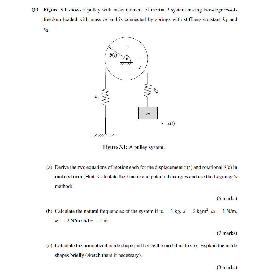
Figure 3.1 shows a pulley with mass moment of inertia J system having two-degrees-of-freedom loaded with mass m and is connected by springs with stiffness constant k1 and k2. (a) D... Figure 3.1 shows a pulley with mass moment of inertia J system having two-degrees-of-freedom loaded with mass m and is connected by springs with stiffness constant k1 and k2. (a) Derive the two equations of motion each for the displacement x(t) and rotational θ(t) in matrix form. (b) Calculate the natural frequencies of the system if m = 1 kg, J = 2 kgm², k1 = 1 N/m, k2 = 2 N/m and r = 1 m. (c) Calculate the normalized mode shape and hence the modal matrix B. Explain the mode shapes briefly. Read more

Steps to Solve

1. Define Kinetic and Potential Energy
   The total kinetic energy ( T ) of the system can be expressed as:
   $$ T = \frac{1}{2} m \dot{x}^2 + \frac{1}{2} J \dot{\theta}^2 $$
   The potential energy ( V ) can be given by the spring forces:
   $$ V = \frac{1}{2} k_1 x^2 + \frac{1}{2} k_2 \left( r\theta \right)^2 $$

2. Apply Lagrange's Equation
   Using Lagrange’s equation:
   $$ \frac{d}{dt}\left(\frac{\partial T}{\partial \dot{q}_i}\right) - \frac{\partial T}{\partial q_i} + \frac{\partial V}{\partial q_i} = 0 $$
   where ( q_1 = x, q_2 = \theta ).

   For ( q_1 = x ):
   $$ m\ddot{x} = -k_1 x - k_2 r \dot{\theta} $$

   For ( q_2 = \theta ):
   $$ J \ddot{\theta} = -k_2 r \theta + k_2 r \frac{\dot{x}}{r} $$

3. Construct the Equations of Motion in Matrix Form
   The resulting equations can be written in matrix form as:
   $$ \begin{bmatrix} m & 0 \ 0 & J \end{bmatrix} \begin{bmatrix} \ddot{x} \ \ddot{\theta} \end{bmatrix} + \begin{bmatrix} k_1 + k_2 & 0 \ 0 & k_2 r^2 \end{bmatrix} \begin{bmatrix} x \ \theta \end{bmatrix} = 0 $$

4. Substitute Parameter Values for Natural Frequencies
   Given ( m = 1 , \text{kg}, , J = 2 , \text{kgm}^2, , k_1 = 1 , \text{N/m}, , k_2 = 2 , \text{N/m}, , r = 1 , \text{m} ):
   The natural frequencies ( \omega ) can be calculated from the determinant equation:
   $$ \text{det}\left(\begin{bmatrix} m\omega^2 + k_1 + k_2 & 0 \ 0 & J\omega^2 - k_2 r^2 \end{bmatrix}\right) = 0 $$

5. Solve the Determinant
   The characteristic equation simplifies to:
   $$ (m\omega^2 + (k_1 + k_2))(J\omega^2 - k_2 r^2) = 0 $$
   Solving gives:
   $$ \omega_1^2 = \frac{k_1 + k_2}{m} , , , \omega_2^2 = \frac{k_2 r^2}{J} $$

6. Calculate Natural Frequencies
   Using the values provided:
   $$ \omega_1^2 = \frac{1 + 2}{1} = 3 \Rightarrow \omega_1 = \sqrt{3} $$
   $$ \omega_2^2 = \frac{2 \times 1^2}{2} = 1 \Rightarrow \omega_2 = 1 $$

7. Determine Normalized Mode Shape and Modal Matrix
   The normalized mode shapes can be calculated by solving the eigenvalue problem, leading to the modal matrix:
   $$ B = \begin{bmatrix} \phi_1 & \phi_2 \end{bmatrix} $$
   The mode shapes will usually correspond to the shapes that the system oscillates in at the natural frequencies.