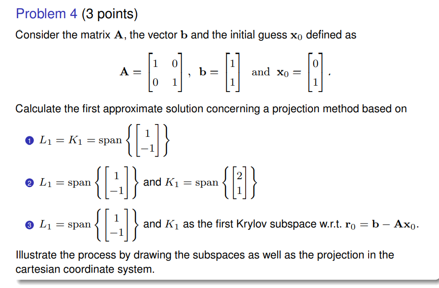
Consider the matrix A, the vector b and the initial guess x0 defined as A = [[1, 0], [0, 1]], b = [[1], [1]] and x0 = [[0], [1]]. Calculate the first approximate solution concer... Consider the matrix A, the vector b and the initial guess x0 defined as A = [[1, 0], [0, 1]], b = [[1], [1]] and x0 = [[0], [1]]. Calculate the first approximate solution concerning a projection method based on: 1) L1 = K1 = span {[[1], [-1]]} 2) L1 = span {[[1], [-1]]} and K1 = span {[[2], [1]]} 3) L1 = span {[[1], [-1]]} and K1 as the first Krylov subspace w.r.t. r0 = b - Ax0. Illustrate the process by drawing the subspaces as well as the projection in the cartesian coordinate system. Read more

Steps to Solve

1. Find the equation for $x_1$

The approximate solution $x_1$ can be written as: $x_1 = x_0 + \delta_1$, where $\delta_1 \in K_1$. The residual vector $r_1 = b - Ax_1$ must be orthogonal to $L_1$, which leads to the Galerkin condition: $L_1^T r_1 = 0$. Substituting $x_1$, we have $r_1 = b - A(x_0 + \delta_1) = b - Ax_0 - A\delta_1$. Therefore, the Galerkin condition becomes $L_1^T(b - Ax_0 - A\delta_1) = 0$, which simplifies to $L_1^T A \delta_1 = L_1^T(b - Ax_0)$. Let $K_1 = span{k_1}$ and $L_1 = span{l_1}$. Then $\delta_1 = \alpha k_1$ for some scalar $\alpha$. The Galerkin condition can be written as $l_1^T A (\alpha k_1) = l_1^T(b - Ax_0)$, which gives us $\alpha = \frac{l_1^T(b - Ax_0)}{l_1^T A k_1}$. Having found $\alpha$, we can find $\delta_1 = \alpha k_1$ and then $x_1 = x_0 + \delta_1$.

2. Solve for case 1: $L_1 = K_1 = span{ \begin{bmatrix} 1 \ -1 \end{bmatrix} }$

Here, $l_1 = k_1 = \begin{bmatrix} 1 \ -1 \end{bmatrix}$. We also have $A = \begin{bmatrix} 1 & 0 \ 0 & 1 \end{bmatrix}$, $b = \begin{bmatrix} 1 \ 1 \end{bmatrix}$, and $x_0 = \begin{bmatrix} 0 \ 1 \end{bmatrix}$. First, calculate $b - Ax_0 = \begin{bmatrix} 1 \ 1 \end{bmatrix} - \begin{bmatrix} 1 & 0 \ 0 & 1 \end{bmatrix} \begin{bmatrix} 0 \ 1 \end{bmatrix} = \begin{bmatrix} 1 \ 1 \end{bmatrix} - \begin{bmatrix} 0 \ 1 \end{bmatrix} = \begin{bmatrix} 1 \ 0 \end{bmatrix}$. Next, calculate $\alpha = \frac{l_1^T(b - Ax_0)}{l_1^T A k_1} = \frac{\begin{bmatrix} 1 & -1 \end{bmatrix} \begin{bmatrix} 1 \ 0 \end{bmatrix}}{\begin{bmatrix} 1 & -1 \end{bmatrix} \begin{bmatrix} 1 & 0 \ 0 & 1 \end{bmatrix} \begin{bmatrix} 1 \ -1 \end{bmatrix}} = \frac{1}{\begin{bmatrix} 1 & -1 \end{bmatrix} \begin{bmatrix} 1 \ -1 \end{bmatrix}} = \frac{1}{1 + 1} = \frac{1}{2}$. Now we have $\delta_1 = \alpha k_1 = \frac{1}{2} \begin{bmatrix} 1 \ -1 \end{bmatrix} = \begin{bmatrix} 1/2 \ -1/2 \end{bmatrix}$. Finally, $x_1 = x_0 + \delta_1 = \begin{bmatrix} 0 \ 1 \end{bmatrix} + \begin{bmatrix} 1/2 \ -1/2 \end{bmatrix} = \begin{bmatrix} 1/2 \ 1/2 \end{bmatrix}$.

3. Solve for case 2: $L_1 = span{ \begin{bmatrix} 1 \ -1 \end{bmatrix} }$ and $K_1 = span{ \begin{bmatrix} 2 \ 1 \end{bmatrix} }$

Here, $l_1 = \begin{bmatrix} 1 \ -1 \end{bmatrix}$ and $k_1 = \begin{bmatrix} 2 \ 1 \end{bmatrix}$. As before, $b - Ax_0 = \begin{bmatrix} 1 \ 0 \end{bmatrix}$.

Now, calculate $\alpha = \frac{l_1^T(b - Ax_0)}{l_1^T A k_1} = \frac{\begin{bmatrix} 1 & -1 \end{bmatrix} \begin{bmatrix} 1 \ 0 \end{bmatrix}}{\begin{bmatrix} 1 & -1 \end{bmatrix} \begin{bmatrix} 1 & 0 \ 0 & 1 \end{bmatrix} \begin{bmatrix} 2 \ 1 \end{bmatrix}} = \frac{1}{\begin{bmatrix} 1 & -1 \end{bmatrix} \begin{bmatrix} 2 \ 1 \end{bmatrix}} = \frac{1}{2 - 1} = \frac{1}{1} = 1$.

Then, $\delta_1 = \alpha k_1 = 1 * \begin{bmatrix} 2 \ 1 \end{bmatrix} = \begin{bmatrix} 2 \ 1 \end{bmatrix}$. Finally, $x_1 = x_0 + \delta_1 = \begin{bmatrix} 0 \ 1 \end{bmatrix} + \begin{bmatrix} 2 \ 1 \end{bmatrix} = \begin{bmatrix} 2 \ 2 \end{bmatrix}$.

4. Solve for case 3: $L_1 = span{ \begin{bmatrix} 1 \ -1 \end{bmatrix} }$ and $K_1$ as the first Krylov subspace w.r.t. $r_0 = b - Ax_0$

Here, $l_1 = \begin{bmatrix} 1 \ -1 \end{bmatrix}$ and $K_1 = span{r_0}$. We already know $r_0 = b - Ax_0 = \begin{bmatrix} 1 \ 0 \end{bmatrix}$, so $k_1 = \begin{bmatrix} 1 \ 0 \end{bmatrix}$.

Now, calculate $\alpha = \frac{l_1^T(b - Ax_0)}{l_1^T A k_1} = \frac{\begin{bmatrix} 1 & -1 \end{bmatrix} \begin{bmatrix} 1 \ 0 \end{bmatrix}}{\begin{bmatrix} 1 & -1 \end{bmatrix} \begin{bmatrix} 1 & 0 \ 0 & 1 \end{bmatrix} \begin{bmatrix} 1 \ 0 \end{bmatrix}} = \frac{1}{\begin{bmatrix} 1 & -1 \end{bmatrix} \begin{bmatrix} 1 \ 0 \end{bmatrix}} = \frac{1}{1} = 1$.

Then, $\delta_1 = \alpha k_1 = 1 * \begin{bmatrix} 1 \ 0 \end{bmatrix} = \begin{bmatrix} 1 \ 0 \end{bmatrix}$. Finally, $x_1 = x_0 + \delta_1 = \begin{bmatrix} 0 \ 1 \end{bmatrix} + \begin{bmatrix} 1 \ 0 \end{bmatrix} = \begin{bmatrix} 1 \ 1 \end{bmatrix}$.

5. Illustrate the process by drawing the subspaces and projection

Since providing a drawing here is not possible, I'll describe what the drawing should contain for each case:

Case 1:

• Draw the vector $x_0 = \begin{bmatrix} 0 \ 1 \end{bmatrix}$.
• Draw the line representing $K_1 = span{ \begin{bmatrix} 1 \ -1 \end{bmatrix} }$.
• Draw the vector $\delta_1 = \begin{bmatrix} 1/2 \ -1/2 \end{bmatrix}$ along the line $K_1$.
• Draw the vector $x_1 = \begin{bmatrix} 1/2 \ 1/2 \end{bmatrix}$ as the sum of $x_0$ and $\delta_1$.

Case 2:

• Draw the vector $x_0 = \begin{bmatrix} 0 \ 1 \end{bmatrix}$.
• Draw the line representing $K_1 = span{ \begin{bmatrix} 2 \ 1 \end{bmatrix} }$.
• Draw the vector $\delta_1 = \begin{bmatrix} 2 \ 1 \end{bmatrix}$ along the line $K_1$.
• Draw the vector $x_1 = \begin{bmatrix} 2 \ 2 \end{bmatrix}$ as the sum of $x_0$ and $\delta_1$.

Case 3:

• Draw the vector $x_0 = \begin{bmatrix} 0 \ 1 \end{bmatrix}$.
• Draw the line representing $K_1 = span{ \begin{bmatrix} 1 \ 0 \end{bmatrix} }$.
• Draw the vector $\delta_1 = \begin{bmatrix} 1 \ 0 \end{bmatrix}$ along the line $K_1$.
• Draw the vector $x_1 = \begin{bmatrix} 1 \ 1 \end{bmatrix}$ as the sum of $x_0$ and $\delta_1$.