Part B (70 points) The first 5 questions each gives you up to 12 points, the last (difficult) question gives you up to 10 points. To get full points your answers must be supported... Part B (70 points) The first 5 questions each gives you up to 12 points, the last (difficult) question gives you up to 10 points. To get full points your answers must be supported by formal arguments. (i) What are the definitions of DRTS, CRTS and IRTS? Sketch a graph of the cost function for each case. The production function is f(x1, x2) = x1x2. Input prices are w₁ > 0 and W2 > 0. We refer to this production function in all questions below. Present some isoquants for this production function. Does the production function f exhibit DRTS, CRTS or IRTS? (explain carefully yours answer). Find MP₁ for f and illustrate. Is MP₁ decreasing? (explain carefully your answer). (ii) With the level of factor 2 fixed at 12 > 0, find the short run cost function as well as (short run) AC, AVC and MC. Illustrate. (iii) In the short run, how will a quantity tax, t > 0, on the product of the producer affect the price he receives (after tax)? How will it affect the consumers? What will be the deadweight loss of such a tax. Illustrate and explain your answer. (iv) Find the long run cost function as well as average and marginal costs. Illustrate. Find the level of output y such that LAC(y) = SAC(y) (long run average cost is equal to short run average cost). Explain and illustrate. (v) Suppose the firm acts as a monopoly facing the demand function D(p) = Ap-4/3 and with both inputs being fully flexible (so in the long run). Illustrate the demand curve. Find revenue as a function of y and illustrate this together with the cost function. Is there a solution to the firm's profit maximization problem? (Why/why not?) If there is a solution find it and illustrate in a figure with the demand curve, MR and MC. (vi) (A) As in (ii), the level of factor 2 is fixed at 12 = 2. Find numerical examples in terms of the output price, p and factor prices w₁ > 0 and w₂ > 0 such that: • The solution to the producer's profit maximization problem in the short run is to shut down, while in the long run there is no solution to the producer's profit maximization problem. • Neither in the short run nor in the long run is there a solution to the producer's profit maximization problem. • There is a solution, both in the short run and in the long run, to the producer's profit maximization problem. Explain carefully your answers. (B) Suppose D(p) = Ap-4/3 and that the firm acts as a monopoly with both inputs being fully flexible. Is there a solution to the firm's profit maximization problem? (Why/why not?) If there is a solution find it.
Understand the Problem
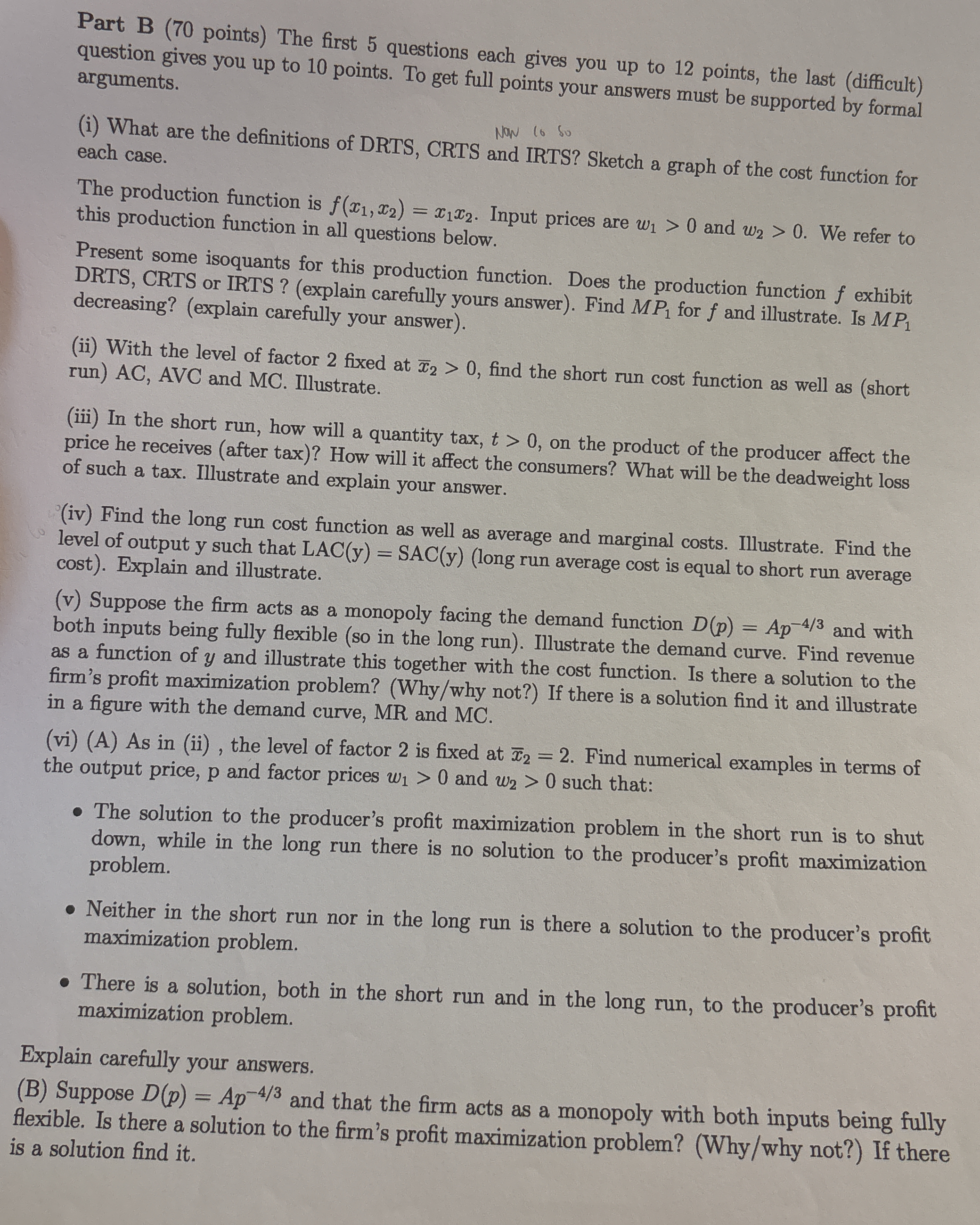
The attached image presents a series of economics questions related to production functions, cost functions, and profit maximization. These questions involve concepts such as DRTS, CRTS, IRTS, isoquants, marginal product, short-run and long-run costs, taxes, deadweight loss, and monopoly behavior. The goal is to solve these problems by finding cost functions, analyzing the impact of taxes, determining profit-maximizing conditions, and illustrating economic concepts graphically.
Answer
(i) DRTS, CRTS, IRTS definitions and graphs. $f(x_1, x_2) = x_1x_2$ exhibits IRTS. $MP_1 = x_2$, not decreasing. (ii) $C(y, \overline{x}_2) = \frac{w_1y}{\overline{x}_2} + w_2\overline{x}_2$, $AC = \frac{w_1}{\overline{x}_2} + \frac{w_2\overline{x}_2}{y}$, $AVC = \frac{w_1}{\overline{x}_2}$, $MC = \frac{w_1}{\overline{x}_2}$. (iii) Quantity tax increases consumer price, decreases producer price, creates deadweight loss. (iv) $C(y) = 2\sqrt{w_1w_2y}$, $LAC = 2\sqrt{\frac{w_1w_2}{y}}$, $LMC = \sqrt{\frac{w_1w_2}{y}}$, $LAC(y) = SAC(y)$ when $y = \overline{x}_2^2$. (v) $R(y) = A^{3/4}y^{1/4}$, $y = \frac{A^3}{256w_1^2w_2^2}$ (vi) (A) Examples provided above. (B) Solution exists
Answer for screen readers
(i) Definitions of DRTS, CRTS, and IRTS are provided above. Graph sketches would show cost functions with convex, linear, and concave shapes, respectively.
Isoquants for $f(x_1, x_2) = x_1x_2$ are rectangular hyperbolas. The production function exhibits IRTS. $MP_1 = x_2$, and it is not decreasing in $x_1$.
(ii) Short-run cost function: $C(y, \overline{x}_2) = \frac{w_1y}{\overline{x}_2} + w_2\overline{x}_2$. $AC = \frac{w_1}{\overline{x}_2} + \frac{w_2\overline{x}_2}{y}$, $AVC = \frac{w_1}{\overline{x}_2}$, $MC = \frac{w_1}{\overline{x}_2}$.
(iii) A quantity tax increases the price paid by consumers and decreases the price received by producers, decreasing equilibrium quantity and creating a deadweight loss.
(iv) Long-run cost function: $C(y) = 2\sqrt{w_1w_2y}$. $LAC = 2\sqrt{\frac{w_1w_2}{y}}$, $LMC = \sqrt{\frac{w_1w_2}{y}}$. $LAC(y) = SAC(y)$ when $y = \overline{x}_2^2$.
(v) Revenue function: $R(y) = A^{3/4}y^{1/4}$. The profit maximization problem has a solution: $y = \frac{A^3}{256w_1^2w_2^2}$
(vi) (A) Examples are in the steps above. (B) There is a solution to the profit maximization problem.
Steps to Solve
- Define DRTS, CRTS, and IRTS and sketch cost functions
- DRTS (Decreasing Returns to Scale): If we multiply all inputs by a factor $k > 1$, output increases by a factor less than $k$. The cost function increases more than proportionally with output. Cost function is convex.
- CRTS (Constant Returns to Scale): If we multiply all inputs by a factor $k > 1$, output increases by a factor of exactly $k$. The cost function increases proportionally with output. Cost function is linear.
- IRTS (Increasing Returns to Scale): If we multiply all inputs by a factor $k > 1$, output increases by a factor more than $k$. The cost function increases less than proportionally with output. Cost function is concave.
- Isoquants for $f(x_1, x_2) = x_1x_2$
Isoquants are curves showing all possible combinations of inputs $x_1$ and $x_2$ that yield the same level of output $y$.
$y = x_1x_2 \implies x_2 = \frac{y}{x_1}$. These are rectangular hyperbolas.
- Returns to scale of $f(x_1, x_2) = x_1x_2$
Let's multiply both inputs by $k > 1$:
$f(kx_1, kx_2) = (kx_1)(kx_2) = k^2x_1x_2 = k^2y$
Since $k^2 > k$ when $k > 1$, the production function exhibits Increasing Returns to Scale (IRTS).
- Marginal Product of $x_1$ ($MP_1$)
$MP_1 = \frac{\partial f}{\partial x_1} = \frac{\partial (x_1x_2)}{\partial x_1} = x_2$
$MP_1$ is the change in output resulting from a small change in input $x_1$, holding $x_2$ constant.
- Is $MP_1$ decreasing?
Since $MP_1 = x_2$, it is constant with respect to $x_1$. Thus, $MP_1$ is not decreasing in $x_1$, given $x_2$ is fixed.
- Short-run cost function with $\overline{x}_2$ fixed
We have $y = x_1\overline{x}_2$, so $x_1 = \frac{y}{\overline{x}_2}$.
The short-run cost function is: $C(y, \overline{x}_2) = w_1x_1 + w_2\overline{x}_2 = w_1\frac{y}{\overline{x}_2} + w_2\overline{x}_2$
- Short-run AC, AVC, and MC
- $AC = \frac{C(y, \overline{x}_2)}{y} = \frac{w_1}{\overline{x}_2} + \frac{w_2\overline{x}_2}{y}$
- $AVC = \frac{w_1y/\overline{x}_2}{y} = \frac{w_1}{\overline{x}_2}$
- $MC = \frac{\partial C(y, \overline{x}_2)}{\partial y} = \frac{w_1}{\overline{x}_2}$
- Quantity tax in the short run
A quantity tax $t > 0$ increases the cost of production. The producer receives $p - t$ per unit sold, where $p$ is the price the consumer pays. The producer's supply curve shifts upward by the amount of the tax. The price paid by consumers increases, and the price received by producers decreases. The equilibrium quantity decreases.
- Deadweight loss of the tax
The deadweight loss is the loss of economic efficiency that occurs when the equilibrium for a good or service is not Pareto optimal. This is represented by a triangle on the graph where the tax is applied.
- Long-run cost function
We need to minimize $w_1x_1 + w_2x_2$ subject to $x_1x_2 = y$. From $x_1x_2 = y$, we have $x_2 = \frac{y}{x_1}$. Substitute into the cost function:
$C = w_1x_1 + w_2\frac{y}{x_1}$
Take the derivative with respect to $x_1$ and set to zero: $\frac{\partial C}{\partial x_1} = w_1 - \frac{w_2y}{x_1^2} = 0 \implies x_1^2 = \frac{w_2y}{w_1} \implies x_1 = \sqrt{\frac{w_2y}{w_1}}$
$x_2 = \frac{y}{x_1} = \frac{y}{\sqrt{\frac{w_2y}{w_1}}} = \sqrt{\frac{w_1y}{w_2}}$
$C(y) = w_1\sqrt{\frac{w_2y}{w_1}} + w_2\sqrt{\frac{w_1y}{w_2}} = \sqrt{w_1w_2y} + \sqrt{w_1w_2y} = 2\sqrt{w_1w_2y}$
- Long-run AC and MC
- $LAC = \frac{C(y)}{y} = \frac{2\sqrt{w_1w_2y}}{y} = 2\sqrt{\frac{w_1w_2}{y}}$
- $LMC = \frac{\partial C(y)}{\partial y} = \frac{2\sqrt{w_1w_2}}{2\sqrt{y}} = \sqrt{\frac{w_1w_2}{y}}$
- $LAC(y) = SAC(y)$
$2\sqrt{\frac{w_1w_2}{y}} = \frac{w_1}{\overline{x}_2} + \frac{w_2\overline{x}_2}{y}$
This is minimized when $y = \overline{x}_2^2$, meaning $x_1 = \overline{x}_2$.
- Monopoly with demand $D(p) = Ap^{-4/3}$
Revenue $R(p) = p \cdot D(p) = Ap^{-1/3}$
To express revenue as a function of $y$, we need to find the inverse demand function. $y = Ap^{-4/3} \implies p^{-4/3} = \frac{y}{A} \implies p = (\frac{y}{A})^{-3/4} = A^{3/4}y^{-3/4}$
Revenue as a function of $y$: $R(y) = p \cdot y = A^{3/4}y^{-3/4} \cdot y = A^{3/4}y^{1/4}$
- Profit maximization for the monopoly
Profit = Revenue - Cost: $\pi(y) = R(y) - C(y) = A^{3/4}y^{1/4} - 2\sqrt{w_1w_2y}$
$\frac{\partial \pi}{\partial y} = \frac{1}{4}A^{3/4}y^{-3/4} - \frac{2\sqrt{w_1w_2}}{2\sqrt{y}} = \frac{1}{4}A^{3/4}y^{-3/4} - \sqrt{\frac{w_1w_2}{y}} = 0$
$\frac{A^{3/4}}{4y^{3/4}} = \sqrt{\frac{w_1w_2}{y}} \implies \frac{A^{3/2}}{16y^{3/2}} = \frac{w_1w_2}{y} \implies A^{3/2}y = 16w_1w_2y^{3/2} \implies y^{1/2} = \frac{A^{3/2}}{16w_1w_2}$
$y = (\frac{A^{3/2}}{16w_1w_2})^2 = \frac{A^3}{256w_1^2w_2^2}$
- (vi)(A) Numerical examples with $\overline{x}_2 = 2$
-
Shutdown in short run, no solution in long run: Short run profit: $\pi = py - w_1x_1 - w_2\overline{x}_2 = p(\overline{x}_2x_1) - w_1x_1 - w_2\overline{x}_2$. Shutdown if $p\overline{x}_2 < w_1$ i.e. revenue cannot cover variable costs. $2p < w_1$.
Long run profit: $\pi = py - 2\sqrt{w_1w_2y}$. To have no solution, the costs must always exceed revenue. The firm should shut down. Example: $p = 1, w_1 = 3, w_2 = 1$. Short run: $2(1) < 3$. Long run: $y - 2\sqrt{3y}$. There is no solution to the profit maximization problem.
-
No solution in either short run or long run: If $p = 0$, there is never a solution. Example: $p = 0, w_1 = 1, w_2 = 1$
-
Solution in both short run and long run: Example: $p = 10, w_1 = 1, w_2 = 1$. Short run: Maximize $10y - x_1 - 2$ where $y = 2x_1$. $10(2x_1) - x_1 - 2$. $20x_1 - x_1 - 2$. $19x_1 - 2$. $x_1 \rightarrow \infty$, so produce infinite output Long run: Maximize $10y - 2\sqrt{y}$.
- (vi)(B) Monopoly with demand $D(p) = Ap^{-4/3}$
As calculated before there is a solution to the profit maximization problem.
(i) Definitions of DRTS, CRTS, and IRTS are provided above. Graph sketches would show cost functions with convex, linear, and concave shapes, respectively.
Isoquants for $f(x_1, x_2) = x_1x_2$ are rectangular hyperbolas. The production function exhibits IRTS. $MP_1 = x_2$, and it is not decreasing in $x_1$.
(ii) Short-run cost function: $C(y, \overline{x}_2) = \frac{w_1y}{\overline{x}_2} + w_2\overline{x}_2$. $AC = \frac{w_1}{\overline{x}_2} + \frac{w_2\overline{x}_2}{y}$, $AVC = \frac{w_1}{\overline{x}_2}$, $MC = \frac{w_1}{\overline{x}_2}$.
(iii) A quantity tax increases the price paid by consumers and decreases the price received by producers, decreasing equilibrium quantity and creating a deadweight loss.
(iv) Long-run cost function: $C(y) = 2\sqrt{w_1w_2y}$. $LAC = 2\sqrt{\frac{w_1w_2}{y}}$, $LMC = \sqrt{\frac{w_1w_2}{y}}$. $LAC(y) = SAC(y)$ when $y = \overline{x}_2^2$.
(v) Revenue function: $R(y) = A^{3/4}y^{1/4}$. The profit maximization problem has a solution: $y = \frac{A^3}{256w_1^2w_2^2}$
(vi) (A) Examples are in the steps above. (B) There is a solution to the profit maximization problem.
More Information
This problem covers a lot of ground in microeconomics, including production functions, cost functions, and monopoly behavior. It requires a solid understanding of calculus and optimization techniques.
Tips
- Confusing returns to scale with diminishing marginal product. Returns to scale refers to what happens when all inputs are scaled up or down, while diminishing marginal product refers to what happens when only one input is varied.
- Incorrectly calculating derivatives when finding marginal product or marginal cost
- Forgetting to account for fixed costs when calculating average total cost.
- Making algebraic errors when solving for optimal input levels.
AI-generated content may contain errors. Please verify critical information