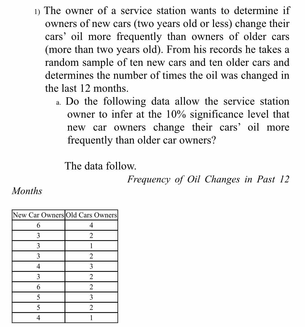
Do the following data allow the service station owner to infer at the 10% significance level that new car owners change their cars' oil more frequently than older car owners? New... Do the following data allow the service station owner to infer at the 10% significance level that new car owners change their cars' oil more frequently than older car owners? New Car Owners: 6, 3, 3, 3, 4, 3, 6, 5, 5, 4 Old Car Owners: 4, 2, 1, 2, 3, 2, 2, 3, 2, 1 Read more

Steps to Solve

1. State the null and alternative hypotheses.

   • Null hypothesis ($H_0$): New car owners change oil with the same frequency as older car owners. $\mu_{new} = \mu_{old}$
   • Alternative hypothesis ($H_1$): New car owners change oil more frequently than older car owners. $\mu_{new} > \mu_{old}$ (right-tailed test)

2. Calculate the means for both samples. $$ \bar{x}{new} = \frac{6+3+3+3+4+3+6+5+5+4}{10} = \frac{42}{10} = 4.2 $$ $$ \bar{x}{old} = \frac{4+2+1+2+3+2+2+3+2+1}{10} = \frac{22}{10} = 2.2 $$

3. Calculate the standard deviations for both samples. $$ s_{new} = \sqrt{\frac{\sum_{i=1}^{10} (x_i - \bar{x}_{new})^2}{n-1}} $$ $$ = \sqrt{\frac{(6-4.2)^2 + (3-4.2)^2 + (3-4.2)^2 + (3-4.2)^2 + (4-4.2)^2 + (3-4.2)^2 + (6-4.2)^2 + (5-4.2)^2 + (5-4.2)^2 + (4-4.2)^2}{10-1}} $$ $$ = \sqrt{\frac{3.24 + 1.44 + 1.44 + 1.44 + 0.04 + 1.44 + 3.24 + 0.64 + 0.64 + 0.04}{9}} $$ $$ = \sqrt{\frac{13.6}{9}} \approx \sqrt{1.511} \approx 1.23 $$

$$ s_{old} = \sqrt{\frac{\sum_{i=1}^{10} (x_i - \bar{x}_{old})^2}{n-1}} $$ $$ = \sqrt{\frac{(4-2.2)^2 + (2-2.2)^2 + (1-2.2)^2 + (2-2.2)^2 + (3-2.2)^2 + (2-2.2)^2 + (2-2.2)^2 + (3-2.2)^2 + (2-2.2)^2 + (1-2.2)^2}{10-1}} $$ $$ = \sqrt{\frac{3.24 + 0.04 + 1.44 + 0.04 + 0.64 + 0.04 + 0.04 + 0.64 + 0.04 + 1.44}{9}} $$ $$ = \sqrt{\frac{7.6}{9}} \approx \sqrt{0.844} \approx 0.92 $$

4. Calculate the t-statistic using the independent samples t-test formula (assuming unequal variances): $$ t = \frac{(\bar{x}{new} - \bar{x}{old}) - (\mu_{new} - \mu_{old})}{\sqrt{\frac{s_{new}^2}{n_{new}} + \frac{s_{old}^2}{n_{old}}}} $$ Since we assume $\mu_{new} - \mu_{old} = 0$ under the null hypothesis: $$ t = \frac{4.2 - 2.2}{\sqrt{\frac{1.23^2}{10} + \frac{0.92^2}{10}}} $$ $$ t = \frac{2}{\sqrt{\frac{1.5129}{10} + \frac{0.8464}{10}}} $$ $$ t = \frac{2}{\sqrt{0.15129 + 0.08464}} = \frac{2}{\sqrt{0.23593}} \approx \frac{2}{0.4857} \approx 4.117 $$

5. Determine the degrees of freedom. Since we are not assuming equal variances, we use the Welch-Satterthwaite equation for approximating df: $$ df \approx \frac{\left(\frac{s_{new}^2}{n_{new}} + \frac{s_{old}^2}{n_{old}}\right)^2}{\frac{\left(\frac{s_{new}^2}{n_{new}}\right)^2}{n_{new}-1} + \frac{\left(\frac{s_{old}^2}{n_{old}}\right)^2}{n_{old}-1}} $$

$$ df \approx \frac{\left(\frac{1.5129}{10} + \frac{0.8464}{10}\right)^2}{\frac{\left(\frac{1.5129}{10}\right)^2}{10-1} + \frac{\left(\frac{0.8464}{10}\right)^2}{10-1}} $$

$$ df \approx \frac{(0.15129 + 0.08464)^2}{\frac{(0.15129)^2}{9} + \frac{(0.08464)^2}{9}} $$

$$ df \approx \frac{(0.23593)^2}{\frac{0.0228886441}{9} + \frac{0.0071649296}{9}} $$

$$ df \approx \frac{0.05566}{0.002543 + 0.000796} = \frac{0.05566}{0.003339} \approx 16.66 $$ Therefore, $df \approx 16$ (rounding down to the nearest integer).

6. Find the critical t-value. For a one-tailed (right-tailed) t-test with $\alpha = 0.10$ and $df = 16$, the critical t-value, $t_{critical}$, is approximately 1.337.

7. Compare the calculated t-statistic to the critical t-value. Since $t = 4.117 > t_{critical} = 1.337$, we reject the null hypothesis.

8. Conclusion:

   At the 10% significance level, there is sufficient evidence to conclude that new car owners change their oil more frequently than older car owners.