Podcast
Questions and Answers
In a histogram, what does the height of each bar typically represent?
In a histogram, what does the height of each bar typically represent?
- The cumulative count of observations up to that value.
- The total number of observations in the dataset.
- The frequency or proportion of observations falling within that bin. (correct)
- The precise value of each observation.
What is the primary purpose of dividing observations into bins when constructing a histogram?
What is the primary purpose of dividing observations into bins when constructing a histogram?
- To represent a true density function of a continuous variable.
- To simplify the data by grouping observations into intervals. (correct)
- To ensure that each observation has a unique representation.
- To allow for easy calculation of the mean and median.
If you increase the number of bins in a histogram, what effect does this have on the display, assuming the data remains the same?
If you increase the number of bins in a histogram, what effect does this have on the display, assuming the data remains the same?
- The overall shape of the distribution remains unchanged.
- The bars become narrower, potentially revealing more detail but also more noise. (correct)
- The histogram becomes a scatterplot.
- The bars become wider, smoothing out the distribution.
Why is it important that each observation in a dataset is allocated to a single bin when creating a histogram?
Why is it important that each observation in a dataset is allocated to a single bin when creating a histogram?
A researcher wants to visualize the distribution of income in a city. Which of the following would be the most appropriate way to present this data to show income density?
A researcher wants to visualize the distribution of income in a city. Which of the following would be the most appropriate way to present this data to show income density?
How does changing the number of bins in a histogram affect the representation of data?
How does changing the number of bins in a histogram affect the representation of data?
For a continuous random variable X with a density function $f_X(x)$, what does the integral $\int_{a}^{b} f_X(x) dx$ represent?
For a continuous random variable X with a density function $f_X(x)$, what does the integral $\int_{a}^{b} f_X(x) dx$ represent?
Why is the probability of a continuous random variable $X$ taking a specific value $x$ (i.e., $P(X = x)$) considered to be zero?
Why is the probability of a continuous random variable $X$ taking a specific value $x$ (i.e., $P(X = x)$) considered to be zero?
Given a small variation $h > 0$, how is the density function $f_X(x)$ for a continuous stochastic variable $X$ related to probability?
Given a small variation $h > 0$, how is the density function $f_X(x)$ for a continuous stochastic variable $X$ related to probability?
The approximation $f_X(x) ≈ P(X = x ± h/2) / h$ is the basis for the definition of which statistical method?
The approximation $f_X(x) ≈ P(X = x ± h/2) / h$ is the basis for the definition of which statistical method?
What is the fundamental question that the Cumulative Distribution Function (CDF) $F_X(t)$ for a continuous variable answers?
What is the fundamental question that the Cumulative Distribution Function (CDF) $F_X(t)$ for a continuous variable answers?
Given a standardized normal distribution, what does $F_X(0) = 0.5$ imply?
Given a standardized normal distribution, what does $F_X(0) = 0.5$ imply?
If $F_X(-1) = 0.159$ for a standardized normal distribution, what percentage of observations have values of x greater than -1?
If $F_X(-1) = 0.159$ for a standardized normal distribution, what percentage of observations have values of x greater than -1?
The cumulative density function (CDF) is defined as $F_X(t) = \int_{-\infty}^{t} f_X(s) ds$. What does $f_X(s)$ represent in this equation?
The cumulative density function (CDF) is defined as $F_X(t) = \int_{-\infty}^{t} f_X(s) ds$. What does $f_X(s)$ represent in this equation?
Which of the following is NOT a property of a Cumulative Distribution Function (CDF)?
Which of the following is NOT a property of a Cumulative Distribution Function (CDF)?
Consider two values, a and b, where a < b. How can you use the CDF, $F_X(x)$, to find the probability that a random variable X falls between a and b?
Consider two values, a and b, where a < b. How can you use the CDF, $F_X(x)$, to find the probability that a random variable X falls between a and b?
Suppose you have a random variable Y and its CDF, $F_Y(t)$. If $F_Y(5) = 0.8$, which of the following statements is the most accurate interpretation?
Suppose you have a random variable Y and its CDF, $F_Y(t)$. If $F_Y(5) = 0.8$, which of the following statements is the most accurate interpretation?
Based on the kernel density plot (kdensity earn, bw(1000)), what can be inferred about the distribution of incomes in the FLEED teaching data?
Based on the kernel density plot (kdensity earn, bw(1000)), what can be inferred about the distribution of incomes in the FLEED teaching data?
If $F_X(t)$ represents the cumulative distribution function (CDF) for a continuous variable X, how would you interpret $F_X(50000)$?
If $F_X(t)$ represents the cumulative distribution function (CDF) for a continuous variable X, how would you interpret $F_X(50000)$?
In the context of kernel density estimation, what is the primary role of the bandwidth parameter?
In the context of kernel density estimation, what is the primary role of the bandwidth parameter?
Given the kernel density plot, what would be the most accurate method to estimate the proportion of the sample with incomes between $20,000 and $60,000?
Given the kernel density plot, what would be the most accurate method to estimate the proportion of the sample with incomes between $20,000 and $60,000?
Suppose you want to compare income distributions across two different years using kernel density estimates. What is the most important consideration when interpreting any observed differences?
Suppose you want to compare income distributions across two different years using kernel density estimates. What is the most important consideration when interpreting any observed differences?
How does the Epanechnikov kernel differ from other kernel functions (e.g., Gaussian) in kernel density estimation?
How does the Epanechnikov kernel differ from other kernel functions (e.g., Gaussian) in kernel density estimation?
Which of the following is a potential drawback of using a very small bandwidth in kernel density estimation?
Which of the following is a potential drawback of using a very small bandwidth in kernel density estimation?
What is the relationship between the kernel density estimator and the histogram?
What is the relationship between the kernel density estimator and the histogram?
Flashcards
Histogram
Histogram
A visualization that shows the distribution of a discrete variable.
Histogram Bar Height
Histogram Bar Height
The height represents the proportion of observations falling into that category.
Histogram Bin
Histogram Bin
A range of values grouped together in a histogram.
Exclusive Bins
Exclusive Bins
Signup and view all the flashcards
Exhaustive Bins
Exhaustive Bins
Signup and view all the flashcards
Bin Adjustment
Bin Adjustment
Signup and view all the flashcards
P(X ∈ A)
P(X ∈ A)
Signup and view all the flashcards
Density Function
Density Function
Signup and view all the flashcards
P(X = x) = 0
P(X = x) = 0
Signup and view all the flashcards
Income Density Plot
Income Density Plot
Signup and view all the flashcards
Kernel Density Estimator
Kernel Density Estimator
Signup and view all the flashcards
Epanechnikov Kernel
Epanechnikov Kernel
Signup and view all the flashcards
Bandwidth in KDE
Bandwidth in KDE
Signup and view all the flashcards
Cumulative Density Function (CDF)
Cumulative Density Function (CDF)
Signup and view all the flashcards
CDF Definition
CDF Definition
Signup and view all the flashcards
CDF Purpose
CDF Purpose
Signup and view all the flashcards
CDF Visual
CDF Visual
Signup and view all the flashcards
What is a Cumulative Density Function (CDF)?
What is a Cumulative Density Function (CDF)?
Signup and view all the flashcards
CDF formula for continuous variables
CDF formula for continuous variables
Signup and view all the flashcards
What does the CDF tell us?
What does the CDF tell us?
Signup and view all the flashcards
CDF Example: FX(-1) for standard normal distribution
CDF Example: FX(-1) for standard normal distribution
Signup and view all the flashcards
CDF Example: FX(0) for standard normal distribution
CDF Example: FX(0) for standard normal distribution
Signup and view all the flashcards
What does the y-axis of a CDF represent?
What does the y-axis of a CDF represent?
Signup and view all the flashcards
What does the x-axis of a CDF represent?
What does the x-axis of a CDF represent?
Signup and view all the flashcards
Study Notes
Logistics
- Bring name placards to class
- Pre-class assignment 1 was due 15 minutes before the class
- Students are allowed up to 2 skips without penalty
- Assignments are graded pass/fail based on effort
- There is an in-class worksheet to complete during the class
- The worksheet must be picked up from the front of the class
- Students can take a photo or scan of the completed worksheet
- The worksheet must be submitted on MyCourses before the next class
- The worksheet is graded pass/fail based on accuracy
Today's Learning Objectives
- Descriptive Statistics
- Including mean, variance, and standard deviation
- Including median and quantiles
- Including density functions
- Including joint distributions
- Sample and Population
- Including representativeness
- Including sampling error
Descriptive Statistics
- Summarisation of information to make data understandable
- The objective is to reduce the amount of numbers while losing as little information as possible
- Stata's summarize command summarises and details data, and allows shortened formats (eg. sum earn, d)
- Descriptive statistics provides key data:
- Sample mean which equals x = n 1/n ΣX(i=1)
- Single number measures of variation
- Selected quantiles
Measures of Variation
- Variance is: Var(x) = 1/n Σ(x-x̄)²
- Standard deviation is: SD(x) = √Var(x)
- Coefficient of variation involves normalizing the standard deviation with the mean to compare across variables:
- CV(x) = SD(x) / x̄
Quantiles
- Quantile Q(p) represents the value below which a fraction p of observations fall
- Some quantiles have specific names, like the median
- Q(.5) is the median, where 50% of observations lie below this value
- Quartiles include Q(.25), Q(.5), and Q(.75)
- Deciles include Q(.1), Q(.2), ..., Q(.9)
- Percentiles include Q(.01), Q(.02), ..., Q(.99)
- The width of a distribution is characterized using percentile ratios
- 90/10 ratio: Q(.9)/Q(.1) = 15
- 90/50 ratio: Q(.9)/Q(.5) = 2.1
- 50/10 ratio: Q(.5)/Q(.1) = 7
Density Functions (Discrete Variables)
- If the distribution of random variable X is discrete, its density function = fX(x) = P(X=x)
- The functions measure the probability that the random variable X takes a specific value x
- Conditions:
- fX(x) ≥ 0
- ∑ fX(x) = 1
- The probability that X takes a value within set A is P(X∈A) = ∑ fX(x) X∈A
- A histogram represents the empirical counterpart of a density function for a discrete variable
Histograms
- The height of each bar in a histogram represents the fraction of observations with a particular value
- The observations are divided into bins to draw a histogram of them
- Each observation is allocated to a single bin, ensuring all observations are assigned
- The width of the bin represents the range of values that observations within that bin can take
- Changing the number of bins allows different perspectives on same data
Density Functions (Continuous Variables)
- The probability that X takes a value within a set A, if X is continuous, is P(X∈A) = ∫ fX(x)dx
- Continuous variables can take infinite values, therefore, X taking a specific value approaches zero P(X=x) = ∫fX(x)dx = 0
- For a probabilistic variable with small variation (h>0):
- fX(x) ≈ P(X=x±h/2)
- (X=x±h/2) means (x - h/2 ≤ X ≤ x+h/2)
- This is the basis for the defintion of a kernel
Kernel Density Estimation
- A kernel density estimator represents a local average for a value - fₙ(x) = 1/n Σ K(x-xᵢ)
- bandwidth (h): Indicates how much data around x is used
- Kernel function (Kₙ): weights observations within the bandwidth
- Stata chooses an “optimal” bandwidth by default
- Larger bandwidth disregards more data
Cumulative Density Function (CDF)
- The CDF for a continuous variable provides the fraction of observations with values of x below t with: Fx(t) = ∫ fX(s)ds
- For instance, in a standardized normal distribution:
- Fx(-1) = 0.159
- Fx(0) = 0.5
- Plotting all of these points will show the entire function for various values of x
Population and Sample
- Population: the entire group of N units about which conclusions are drawn
- Sample: a specific group of n units selected from the population to collect data
- Aim is inference of the population
- This refers to deducing or concluding information from evidence/reasoning instead of explicit statements
- sampling bias: sample must represent population
- sampling error: exceptional observations must be sampled by chance
Sampling Bias: 1936 US Presidential Election Polls
- Literary Digest sent 10 million "straw” ballots, asking who people intended to vote for in the upcoming election
- 2.4 million ballots were returned
- 57% indicated they would vote for Landon
- 43% indicated they would vote for Roosevelt
- Fact: Roosevelt won the election with 62% of the vote
- George Gallup also conducted a poll
- Sample size was just 50,000
- Prediction: 56% for Roosevelt
Sampling Error
- Random sampling removes bias
- each object in population has same probability of being selected into the sample
- difference between a sample statistic and population parameter arising by chance
Sampling Error Example
- The population mean income among 15-64 year olds in Finland in 2010 (N ≈ 3.5M) was €26,144 µx = 1/n Σxᵢ
- Sample Average: x̄ = 1/n Σxᵢ
- The larger the smaple size, the closer the sample average tends to be to the population mean
- Sample averages are distributed relatively symmetrically around population mean
- These Properties are also known as:
- The law of Large Numbers
- Central Limit Theorem
Cross Tabulation (Joint Distribution)
- Table displays small data sets of two variables
- Each observation has:
- Rows = values of Y
- Columns = values of X
- Cells = observations of value (y, x)
- Cross tabulation cells report the share of observations with value (y, x)
- fXY(x, y) = P(X = x, Y = y) shows that the empirical counterpart of the joint density function
- Probability: the random variable X takes the value x and that random variable Y takes the value y
Summary Of Key Concepts
- Concepts
- density function, including CDF
- joint distributions
- Things to worry about when using samples
- representativeness
- sampling error
The next lecture features:
- Conditional descriptive statistics
- and applications to make sense of recent research on inequality
Upcoming Assignments
- In-class worksheet 1 due on MyCourses before next lecture
- You may upload a photo/scan (preferred) OR
- can turn in paper copy in-person beginning of next lecture
- Pre-class assignment 2 = due 15 minutes before next lecture
- Homework 1 = due Jan 15
- attend exercise session 1 for practical tools
- you have the conceptual tools to get started
Studying That Suits You
Use AI to generate personalized quizzes and flashcards to suit your learning preferences.